
Lake Superior State University Team AMORE Drone Simulation: UAV Launch and Recovery with USV
By Tanya Kuruvilla
Published on MATLAB Students Lounge
April 5, 2023
In today’s blog, Team AMORE from Lake Superior State University will share how they used MATLAB to simulate their drone launch and recovery from an unmanned surface vehicle. Over to you, Team AMORE…

Who We Are
Team AMORE is comprised of undergraduate students from Lake Superior State University located in Sault Ste Marie, Michigan. Sault Ste Marie is in Michigan’s Upper Peninsula and is an hour’s drive from three Great Lakes, the closest being Lake Superior. Lake Superior is the largest freshwater lake in the world, which provides a great testing environment for marine robotics. Team Amore (Autonomous Marine Operations and Robotics Engineering) designs vessels to compete in competitions hosted by RoboNation (ex: RobotX & Roboboat) and conducts research. Past research initiatives have been a collaboration with Team AMORE, Lake Superior State University’s Center for Freshwater Research and Education, and conservation biology students. We have partaken in autonomous freshwater quality monitoring, Zooplankton research at Greenwood Nature Sanctuary, and oil spill detection and remediation.
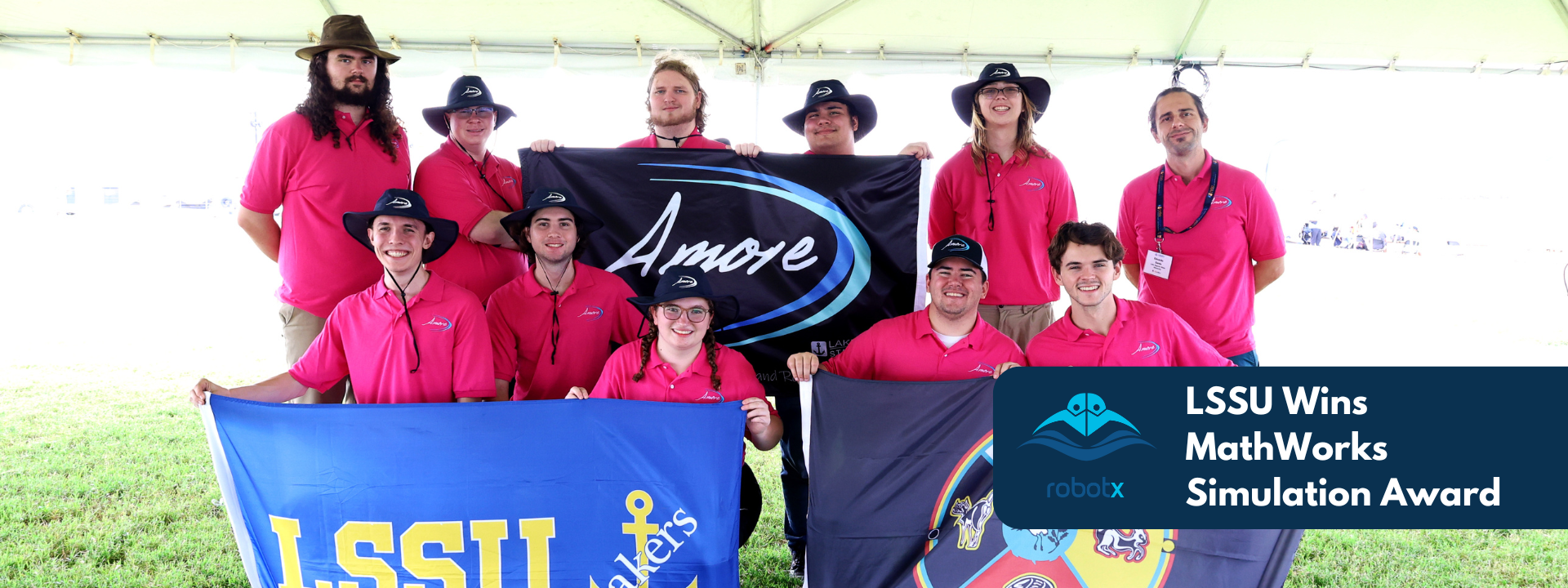
At RobotX 2024, Team AMORE placed first in the MathWorks Simulation Challenge, fourth in technical documentation, and received an award for resiliency.
The Challenge:
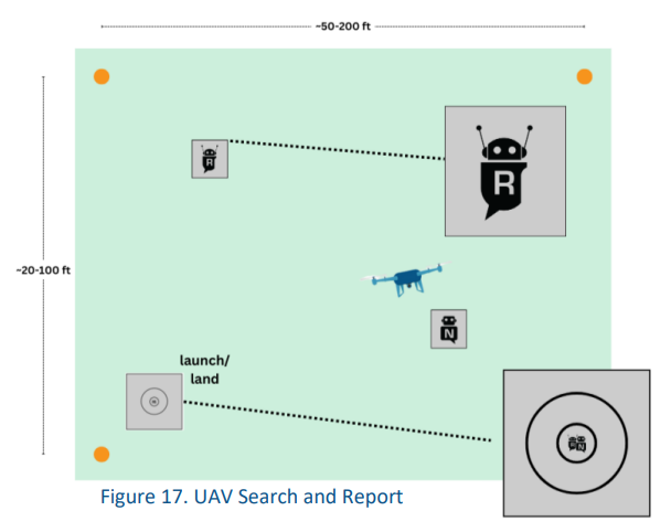
Team AMORE competes in the Maritime RobotX Challenge hosted by RoboNation. The RobotX challenge is comprised of various on-shore technical documentation aspects and 8 autonomy challenges to be completed with an Unmanned Surface Vehicle (WAM-V) and an Unmanned Ariel Vehicle (drone). Team AMORE wanted to integrate an Unmanned Aerial Vehicle (UAV) with our Unmanned Surface Vehicle (USV) to be able to complete the UAV Replenishment and UAV Search & Report tasks for the RobotX competition. The main challenge we faced was the climate of Sault Ste Marie. From October through March, weather such as snow, sleet, hail, and heavy rain limits the amount of outdoor testing that we can accomplish. We had space to test the launch and recovery sequence indoors, but we needed to develop the controller first to ensure that it would act as expected since we would not have time to recover it if things went awry. This is where the tools provided to us by MathWorks come into play.
How did we implement it?
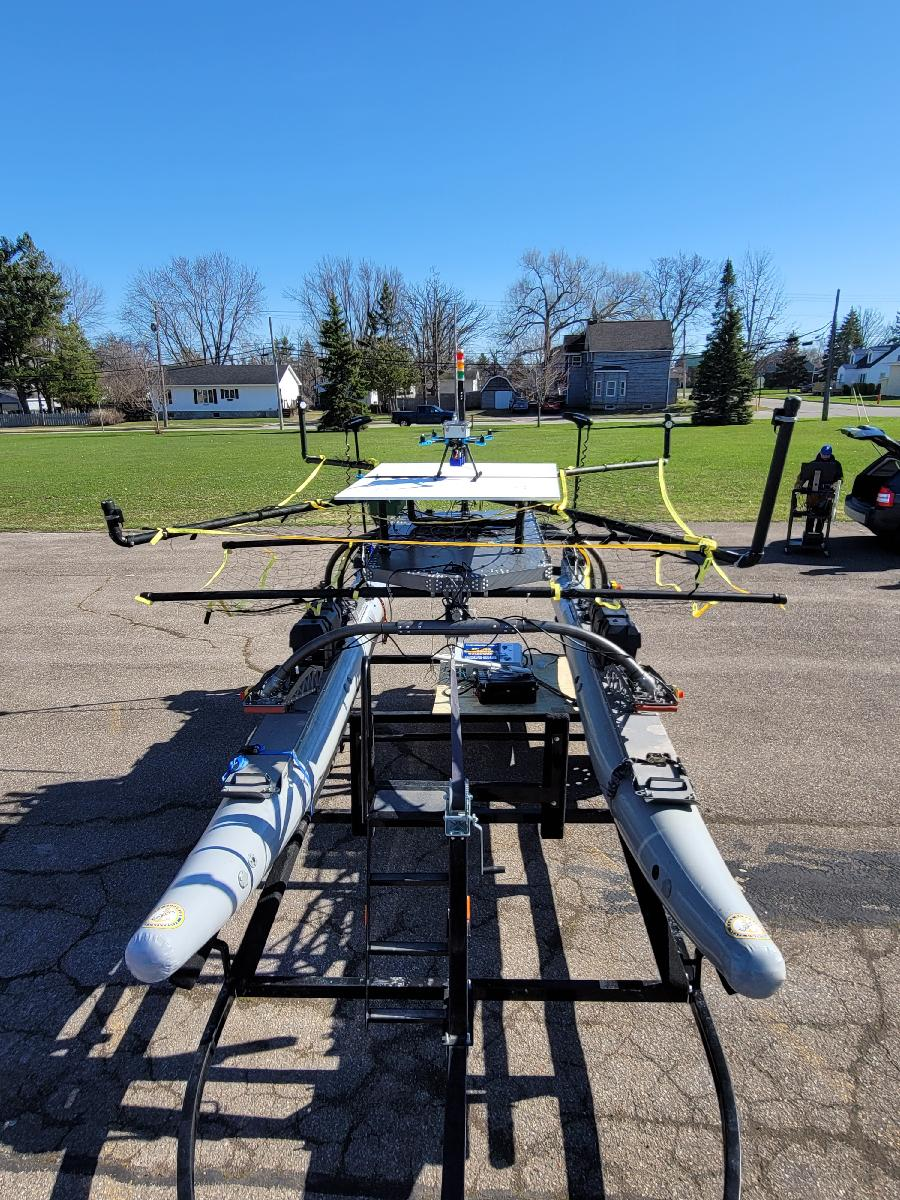
Team AMORE first developed a Landing and Recovery Platform to install on our WAM-V. The landing platform has a base for the drone to land on and arms extending out with netting. On these arms, we have installed Pozyx Indoor GPS anchors to create a local coordinate frame over the USV. This coordinate frame is used by the UAV to accurately land on the Landing and Recovery Platform. This novel approach allows the UAV to land on the USV without any vision system.
Indoor Testing of the UAV
Using MATLAB, we first created a dynamic model for the drone. This model simulated various forces that act on the drone during flight such as wind. We were able to give the motors a desired RPM and would see the UAV respond accordingly. We then were able to develop and tune a PID controller to help the UAV respond to wind or any other disturbances that it would encounter during an outdoor flight. With the drone PID controller functioning as expected, the focus was shifted to developing the dynamic model for the USV which was modeled after the WAM-V. This dynamic model simulated disturbances such as wind and current. With a functioning dynamic model, the PID controller was developed and tuned for the USV. The USV PID controller was set up to replicate the differential thrust configuration used on our WAM-V for long-range navigation. When launched, the UAV would first navigate to a point and then it would follow the USV for a set period of time. Once the time had elapsed, the UAV would initiate the landing sequence and was successfully recovered by the USV.
Results
In MATLAB, we are able to see the path of both unmanned systems during their mission. This simulation allowed us to verify that we could successfully land our UAV on our USV within the area of the landing platform before moving on to real-life testing.
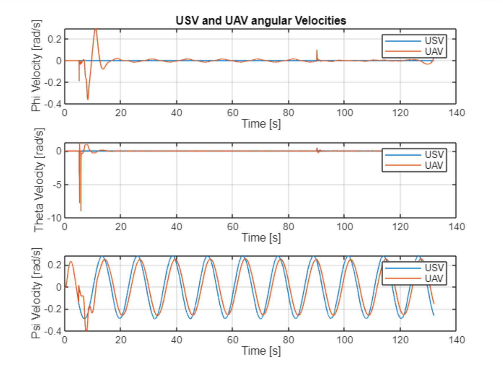
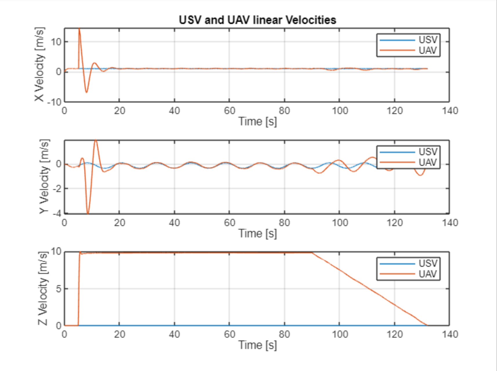
Here, on the left, we have plotted the UAV and USV’s velocities in x, y, and z for the duration of the mission. The angular velocity plot (middle) shows how fast each vehicle is rotating around x,y, and z. After the UAV has reached its waypoint, we want both vehicles to have as close to the same angular velocities as possible since the UAV is essentially mirroring the movements of the USV. The third plot shows the position of both vehicles in x, y, and z during the mission. This can be used to breakdown how high the UAV is flying and if it is actually following the mission along the x,y plane as expected.
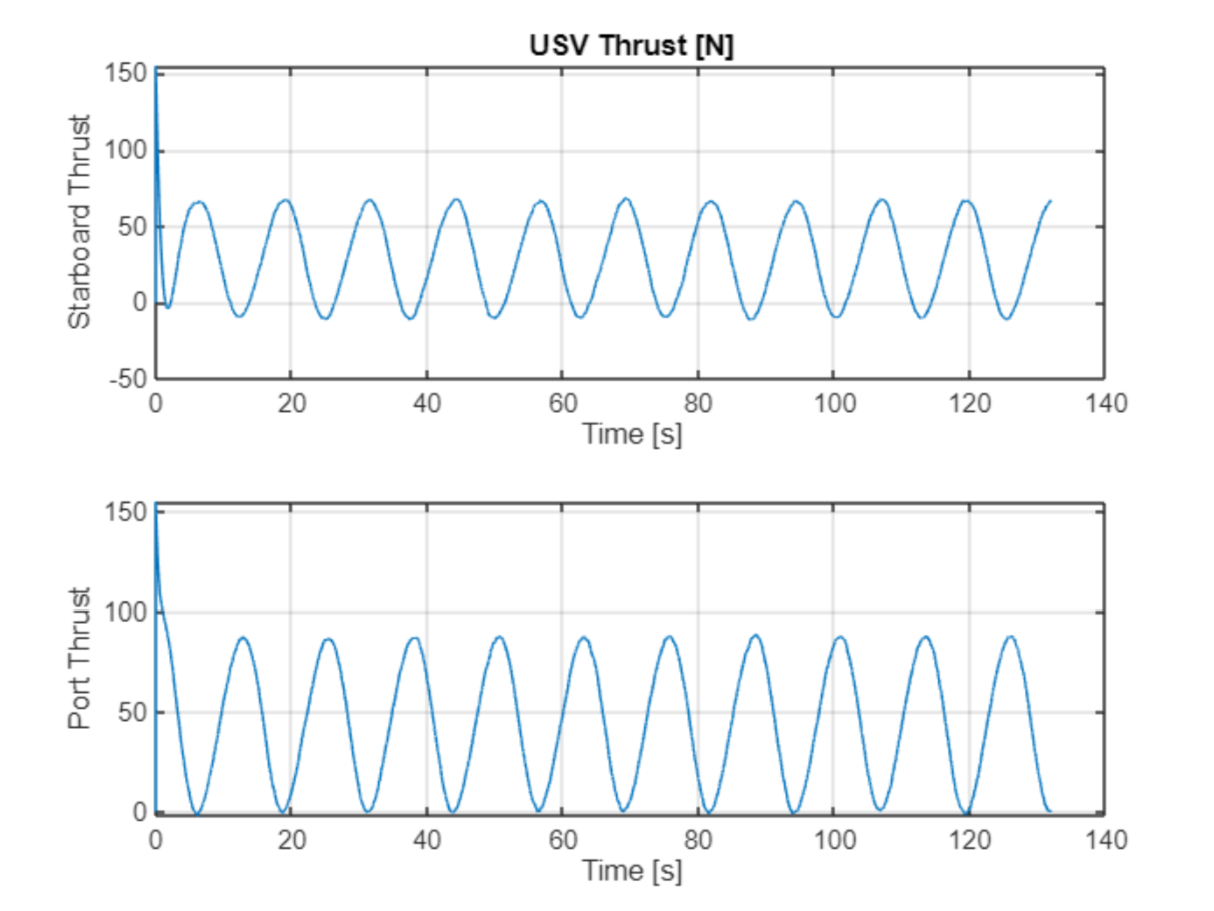
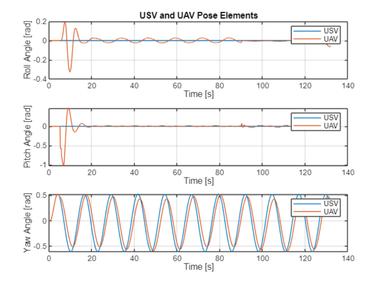
The USV and UAV pose elements plot shows the degree of rotation in x, y, & z for both vehicles over the time of the mission. The movements to achieve those angles are called roll, pitch, and yaw respectively. Since the UAV is trying to follow the heading of the vehicle as well as the position, we would want to see little movement in pitch and roll since it should only need minor adjustments to stay above the USV. We do want to see the yaw angle change to follow the USV’s, as that is the rotation about z, also known as heading. The USV Thrust plot shows thrust for both the starboard and port thrust on the USV. On our WAM-V we use differential thrust, two thrusters of varying state, to achieve the desired positioning.
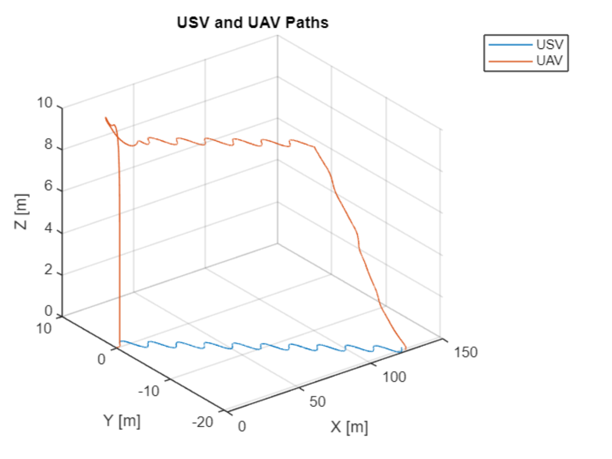
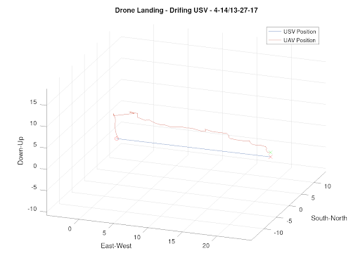
The UAV and USV path plot is the most important plot we developed. The plot shows the USV, or WAM-V, following a sinusoidal path while the UAV takes off from the platform, flys to a point, then lands back onto the WAM-V. The x-error and y-error output by the program is the error between the middle of the landing platform and where it actually landed.
x-error: 0.621m
y-error: 0.790m
Since our platform board is 1×1 meter and the net makes it around 3×3 meters, anything in that range is a successful landing.
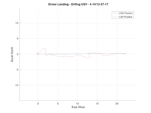
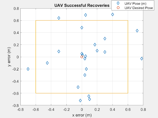
The plots below show the data from in-person testing of the PID controller developed for the UAV in different coordinates and the last graph shows the error in the x and y axes when landing.
This simulation would not have been possible if it wasn’t for MATLAB. The tools and libraries through MATLAB were crucial in the creation and design of the dynamic models and PID controllers. We thank MathWorks for providing us with the tools and the opportunity to showcase our hard work
Read this article on the MatLab Students Blog: